Mathematics for Machine Learning & Data Science¶

1 - Basics of NumPy¶

1.1 Packages¶

import numpy as np

1.2 - NumPy arrays¶

# One dimensional array
one_dimensional_arr = np.array([10, 12])
print(one_dimensional_arr)

# print("\n") # creating space between the output
print()
# Two dimensional array
two_dimensional_arr = np.array(
    [
        [10, 20],
        [30, 40]
    ]
)
print(two_dimensional_arr)

#print("\n")
print()

# Create an array with 3 integers, starting from the default integer 0
# np.arange()
arr_of_three = np.arange(3)
print(arr_of_three)

print()

# Create an arry that starts from the integer 1, and ends at 20, incremented by 3
# np.arange()
arr_inc_by_three = np.arange(1, 20, 3)
print(arr_inc_by_three)

print()

# An array with evenly spaced values
# np.linspace()
# Default type for values in the NumPy fun np.linspace() is floating (np.float64)
arr_with_evenSpace = np.linspace(0, 100, 5)
print(arr_with_evenSpace)

print()

# Change the dtype to Integers np.linspace()
arr_linSpace_Int = np.linspace(0, 100, 5, dtype=int)
print(arr_linSpace_Int)

print()
# change dtype to float np.arange()
arr_arange_to_float = np.arange(1, 20, 3, dtype=float)
print(arr_arange_to_float)

[10 12]

[[10 20]
 [30 40]]

[0 1 2]

[ 1  4  7 10 13 16 19]

[  0.  25.  50.  75. 100.]

[  0  25  50  75 100]

[ 1.  4.  7. 10. 13. 16. 19.]

1.3 - More on NumPy arrays¶

np.ones() - Returns a new array setting values to one.
np.zeros() - Returns a new array setting values to zero.
np.empty() - Returns a new uninitialized array.
np.random.rand() - Returns a new array with values chosen at random.

# Return a new array of shape 3, filled wirth ones.
import numpy as np
ones_arr = np.ones(3)
print(ones_arr)

print()

# Return a new array of shape 3, filled with zeros
zeros_arr = np.zeros(3)
print(zeros_arr)

print()

# Return a new array of shape 3, with initializing entries
empt_arr = np.empty(3)
print(empt_arr)

print()
# Return a new array of shape 3 with random numbers between 0 and 1
rand_arr = np.random.rand(3)
print(rand_arr)

[1. 1. 1.]

[0. 0. 0.]

[0. 0. 0.]

[0.6462132  0.81140024 0.42673117]

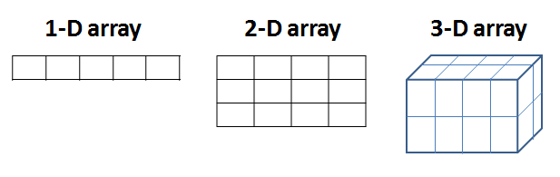
2 - Multidimensional Arrays¶

With NumPy you can also create arrays with more than one dimension. In the above examples, you dealt with 1-D arrays, where you can access their elements using a single index. A multidimensional array has more than one column. Think of a multidimensional array as an excel sheet where each row/column represents a dimension.

2.1 - Finding size, shape and dimension.¶

ndarray.ndim - Stores the number dimensions of the array.
ndarray.shape - Stores the shape of the array. Each number in the tuple denotes the lengths of each corresponding dimension.
ndarray.size - Stores the number of elements in the array.

# Create a 2 dimensional array (d-D)
import numpy as np
two_dim_arr = np.array(
    [
        [1, 2,3 ],
        [4, 5, 6]
    ]
)
print(two_dim_arr)

print()

# An alternative way to create a multidimensional array is by reshaping the 
# 1-D array using 
# np.reshape()

# 1-D array
one_dim_arr = np.array(
    [1, 2, 3, 4, 5, 6, 7, 8, 9]
)
print(one_dim_arr)

print()

# mult dimensional array using np.reshape()
mul_dim_arr = np.reshape(
    one_dim_arr,  # the array to be reshped
    (3, 3) #dimensions of the new array
)
print(mul_dim_arr)

[[1 2 3]
 [4 5 6]]

[1 2 3 4 5 6 7 8 9]

[[1 2 3]
 [4 5 6]
 [7 8 9]]

3 - Array math operations¶

In this section, you will see that NumPy allows you to quickly perform elementwise addition, substraction, multiplication and division for both 1-D and multidimensional arrays. The operations are performed using the math symbol for each ‘+’, ‘-’ and ‘*’. Recall that addition of Python lists works completely differently as it would append the lists, thus making a longer list, in addition, subtraction and multiplication of Python lists do not work.


arr_1 = np.array([2, 4, 6])
arr_2 = np.array([1, 3, 5])

# Adding two 1-D arrays
addition = arr_1 + arr_2
print(addition)

# Subtracting two 1-D arrays
subtraction = arr_1 - arr_2
print(subtraction)

# Multiplying two 1-D arrays elementwise
multiplication = arr_1 * arr_2
print(multiplication)

[ 3  7 11]
[1 1 1]
[ 2 12 30]

3.1 - Multiplying vector with a scalar (broadcasting)¶

Suppose you need to convert miles to kilometers. To do so, you can use the NumPy array functions that you’ve learned so far. You can do this by carrying out an operation between an array (miles) and a single number (the conversion rate which is a scalar). Since, 1 mile = 1.6 km, NumPy computes each multiplication within each cell.

This concept is called broadcasting, which allows you to perform operations specifically on arrays of different shapes.

vector = np.array([1, 2])
vector * 1.6

array([1.6, 3.2])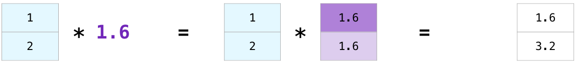

4 - Indexing and slicing¶

Indexing is very useful as it allows you to select specific elements from an array. It also lets you select entire rows/columns or planes as you’ll see in future assignments for multidimensional arrays.

4.1 - Indexing¶

Let us select specific elements from the arrays as given.

# Select the third element of the array. Remember the counting starts from 0.
import numpy as np
a = ([1, 2, 3, 4, 5])
print(a[2])

# Select the first element of the array.
print(a[0])

3
1

# For multidimensional arrays of shape n, to index a specific element, 
# you must input n indices, one for each dimension.

# Indexing an a 2-D array
two_dim = np.array(
    (
        [1, 2, 3],
        [4, 5, 6],
        [7, 8, 9]
    )
)
# Select element number 8 from the 2-D array using indices i, j.
print(two_dim[2][1])

4.2 - Slicing¶

Slicing gives you a sublist of elements that you specify from the array. The slice notation specifies a start and end value, and copies the list from start up to but not including the end (end-exclusive).

The syntax is:

array[start:end:step]

If no value is passed to start, it is assumed start = 0, if no value is passed to end, it is assumed that end = length of array - 1 and if no value is passed to step, it is assumed step = 1.

# Slice the array a to get the array [2,3,4]
a = ([1, 2, 3, 4, 5])
sliced_arr = a[1:4]
print(sliced_arr)

print()

# slice the array a to get the array [1, 2, 3]
sliced_arr = a[:3]
print(sliced_arr)

print()

# Slice the array a to get the array [3, 4, 5]
sliced_arr = a[2:]
print(sliced_arr)

print()

# Slice the array a to get the array [1,3,5]
sliced_arr = a[::2]
print(sliced_arr)

print()
print(a[:])
print(a[::])

print()
# Note that a == a[:] == a[::]
print(a == a[:] == a[::])

print()

# Slice the two_dim array to get the first two rows
print(two_dim)
print()
sliced_arr_1 = two_dim[0:2]
print(sliced_arr_1)

print()

# Similarily, slice the two_dim array to get the last two rows
sliced_two_dim_rows = two_dim[1:3]
print(sliced_two_dim_rows)

print()

sliced_two_dim_col = two_dim[:, 1]
print(sliced_two_dim_col)

[2, 3, 4]

[1, 2, 3]

[3, 4, 5]

[1, 3, 5]

[1, 2, 3, 4, 5]
[1, 2, 3, 4, 5]

True

[[1 2 3]
 [4 5 6]
 [7 8 9]]

[[1 2 3]
 [4 5 6]]

[[4 5 6]
 [7 8 9]]

[2 5 8]

5 - Stacking¶

Finally, stacking is a feature of NumPy that leads to increased customization of arrays. It means to join two or more arrays, either horizontally or vertically, meaning that it is done along a new axis.

np.vstack() - stacks vertically
np.hstack() - stacks horizontally
np.hsplit() - splits an array into several smaller arrays

import numpy as np
a1 = np.array(
    [
        [1,1],
        [2, 2]
    ]
)
a2 = np.array(
    [
        [3,3],
        [4,4]
    ]
)

print(f'a1:\n{a1}')
print(f'a2:\n{a2}')

print()

# Stack the arrays horizontally
horz_stack = np.hstack((a1, a2))
print(horz_stack)

print()

# Stack the arrays vertically
ver_stack = np.vstack((a1, a2))
print(ver_stack)

a1:
[[1 1]
 [2 2]]
a2:
[[3 3]
 [4 4]]

[[1 1 3 3]
 [2 2 4 4]]

[[1 1]
 [2 2]
 [3 3]
 [4 4]]

# How to use np.hsplit()
# Splitting into a specific number of equal parts

import numpy as np

# Create a 3x6 array
arr = np.array(
    [
        [1,2,3,4,5,6],
        [7,8,9,10,11,12],
        [13, 14, 15, 16, 17, 18]
    ]
)
# Split the array into 3 equal horizontal sub-arrays
split_arr = np.hsplit(arr, 3)

print("Original array:\n", arr)
print("\nSplit array (3 parts:\n", split_arr)
print("\nShape of each sub-array:", split_arr[0].shape)

Original array:
 [[ 1  2  3  4  5  6]
 [ 7  8  9 10 11 12]
 [13 14 15 16 17 18]]

Split array (3 parts:
 [array([[ 1,  2],
       [ 7,  8],
       [13, 14]]), array([[ 3,  4],
       [ 9, 10],
       [15, 16]]), array([[ 5,  6],
       [11, 12],
       [17, 18]])]

Shape of each sub-array: (3, 2)

Solving Linear Systems: 2 variables¶

By completing this lab, you will be able to use basic programming skills with Python and NumPy package to solve systems of linear equations. In this notebook you will:

Use NumPy linear algebra package to find the solutions of the system of linear equations
Find the solution for the system of linear equations using elimination method
Evaluate the determinant of the matrix and examine the relationship between matrix singularity and number of solutions of the linear system

Table of Contents¶

1 - Representing and Solving System of Linear Equations using Matrices
- 1.1 - System of Linear Equations
- 1.2 - Solving Systems of Linear Equations using Matrices
- 1.3 - Evaluating Determinant of a Matrix
2 - Solving System of Linear Equations using Elimination Method
- 2.1 - Elimination Method
- 2.2 - Preparation for the Implementation of Elimination Method in the Code
- 2.3 - Implementation of Elimination Method
- 2.4 - Graphical Representation of the Solution
3 - System of Linear Equations with No Solutions
4 - System of Linear Equations with Infinite Number of Solutions

1 - Representing and Solving System of Linear Equations using Matrices¶

1.1 - System of Linear Equations¶

System of Linear Equations¶

A system of linear equations (or a linear system) is a set of two or more linear equations involving the same set of variables. A linear equation is an equation where each term is either a constant or the product of a constant and a single variable raised to the power of 1. There are no products or powers of variables.

A general form of a system of $m$ linear equations in $n$ variables ( $x_1, x_2, ..., x_n$ ) can be written as:

a_{11}x_1 + a_{12}x_2 + ... + a_{1n}x_n = b_1
a_{21}x_1 + a_{22}x_2 + ... + a_{2n}x_n = b_2
...
a_{m1}x_1 + a_{m2}x_2 + ... + a_{mn}x_n = b_m

Where:

$x_1, x_2, ..., x_n$ are the variables (or unknowns).
$a_{ij}$ are the coefficients of the variables (constants). The first subscript $i$ indicates the equation number (from 1 to $m$ ), and the second subscript $j$ indicates the variable number (from 1 to $n$ ).
$b_1, b_2, ..., b_m$ are the constant terms (or the right-hand side values).

Goal:

The goal when dealing with a system of linear equations is to find the values for each of the variables ( $x_1, x_2, ..., x_n$ ) that simultaneously satisfy all the equations in the system.

Solutions to a System of Linear Equations:

A system of linear equations can have one of three possible types of solutions:

Unique Solution: There is exactly one set of values for the variables that satisfies all the equations. Geometrically, in the case of two variables, this corresponds to two lines intersecting at a single point. In three variables, it corresponds to three planes intersecting at a single point.
Infinitely Many Solutions: There are infinitely many sets of values for the variables that satisfy all the equations. This occurs when the equations are dependent on each other. Geometrically, in two variables, this means the two lines are coincident (they are the same line). In three variables, this can happen if the planes intersect in a line or if all the planes are the same.
No Solution: There is no set of values for the variables that can satisfy all the equations simultaneously. The system is said to be inconsistent. Geometrically, in two variables, this means the two lines are parallel and distinct (they never intersect). In three variables, this can occur if planes are parallel or intersect in a way that doesn’t yield a common point.

Methods for Solving Systems of Linear Equations:

Several methods can be used to solve systems of linear equations, including:

Substitution: Solving one equation for one variable and substituting that expression into the other equations.
Elimination (or Addition/Subtraction): Manipulating the equations to eliminate one variable at a time by adding or subtracting multiples of the equations.
Matrix Methods:
- Gaussian Elimination and Gauss-Jordan Elimination: Using elementary row operations on the augmented matrix of the system to transform it into row-echelon form or reduced row-echelon form.
- Matrix Inversion: If the system has the form $AX = B$ and the coefficient matrix $A$ is invertible, the solution is $X = A^{-1}B$ .
- Cramer’s Rule: Using determinants to find the solution for each variable (only applicable when the number of equations equals the number of variables and the determinant of the coefficient matrix is non-zero).
Graphical Methods: For systems with two variables, the solution can be found by plotting the lines corresponding to each equation and finding their point of intersection (if any).

Applications of Systems of Linear Equations:

Systems of linear equations have a wide range of applications in various fields, including:

Mathematics: Solving algebraic problems, finding intersections of geometric objects.
Physics: Analyzing circuits, solving mechanics problems.
Engineering: Designing structures, controlling systems.
Economics: Modeling supply and demand, analyzing market equilibrium.
Computer Science: Solving linear programming problems, computer graphics.
Statistics: Linear regression.

Understanding systems of linear equations is fundamental in many scientific and technical disciplines. The methods for solving them provide powerful tools for analyzing and solving real-world problems.

1.2 - Solving Systems of Linear Equations using Matrices¶

More information about the np.linalg.solve() function can be found in documentation

import numpy as np
# Matrix A
A = np.array(
    [
        [-1, 3],
        [3, 2]
    ]
)
# 1-D array
b = np.array([7, 1], dtype = np.dtype(float))
print("Matrix A:")
print(A)
print("\nArray b:")
print(b)

Matrix A:
[[-1  3]
 [ 3  2]]

Array b:
[7. 1.]

Check the dimensions of and using the shape attribute (you can also use np.shape() as an alternative):

print(f"Shape of A: {A.shape}")
print(f"Shape of b: {b.shape}")

Shape of A: (2, 2)
Shape of b: (2,)

x = np.linalg.solve(A, b)
print(f"Solution: {x}")

Solution: [-1.  2.]

Linear Algebra Solution¶

The given system of linear equations can be represented in matrix form as $Ax = b$ , where:

The coefficient matrix $A$ is:

A = \begin{bmatrix} -1 & 3 \\ 3 & 2 \end{bmatrix}

(1)

The vector of unknowns $x$ is:

x = \begin{bmatrix} x_1 \\ x_2 \end{bmatrix}

(2)

And the constant vector $b$ is:

b = \begin{bmatrix} 7 \\ 1 \end{bmatrix}

(3)

The system of equations is thus: $$

\begin{bmatrix} -1 & 3 \\ 3 & 2 \end{bmatrix}

(4)

\begin{bmatrix} x_1 \\ x_2 \end{bmatrix}

(5)

\begin{bmatrix} 7 \\ 1 \end{bmatrix}

(6)

To solve for $x$ , we can use the formula $x = A^{-1}b$ , provided that the inverse of $A$ exists. The determinant of $A$ is:

\det(A) = (-1)(2) - (3)(3) = -2 - 9 = -11

(7)

Since the determinant is non-zero, the inverse exists.

The inverse of a $2 \times 2$ matrix $\begin{bmatrix} a & b \\ c & d \end{bmatrix}$ is $\frac{1}{ad - bc} \begin{bmatrix} d & -b \\ -c & a \end{bmatrix}$ . Therefore, the inverse of $A$ is: $$ A^{-1} = \frac{1}{-11} \begin{bmatrix} 2 & -3 \ -3 & -1 \end{bmatrix}¶

\begin{bmatrix} -\frac{2}{11} & \frac{3}{11} \\ \frac{3}{11} & \frac{1}{11} \end{bmatrix}

(8)

Now, we can find the solution $x$ : $$ x = A^{-1}b =

\begin{bmatrix} -\frac{2}{11} & \frac{3}{11} \\ \frac{3}{11} & \frac{1}{11} \end{bmatrix}

(9)

\begin{bmatrix} 7 \\ 1 \end{bmatrix}

(10)

\begin{bmatrix} (-\frac{2}{11})(7) + (\frac{3}{11})(1) \\ (\frac{3}{11})(7) + (\frac{1}{11})(1) \end{bmatrix}

(11)

\begin{bmatrix} -\frac{14}{11} + \frac{3}{11} \\ \frac{21}{11} + \frac{1}{11} \end{bmatrix}

(12)

\begin{bmatrix} -\frac{11}{11} \\ \frac{22}{11} \end{bmatrix}

(13)

\begin{bmatrix} -1 \\ 2 \end{bmatrix}

(14)

Thus, the solution to the system of linear equations is $x_1 = -1$ and $x_2 = 2$ .

1.3 - Evaluating Determinant of a Matrix¶

Matrix corresponding to the linear system is a square matrix - it has the same number of rows and columns. In case of a square matrix it is possible to calculate its determinant - a real number which characterizes some properties of the matrix. Linear system containing two (or more) equations with the same number of unknown variables will have one solution if and only if matrix has non-zero determinant.

Let’s calculate the determinant using NumPy linear algebra package. You can do it with the np.linalg.det(A) function. More information about it can be found in documentation.

import numpy as np
d = np.linalg.det(A)
print(f"Determinant of matrix A: {d:.2f}")

Determinant of matrix A: -11.00

2 - Solving System of Linear Equations using Elimination Method¶

You can see how easy it is to use contemporary packages to solve linear equations. However, for deeper understanding of mathematical concepts, it is important to practice some solution techniques manually. Programming approach can still help here to reduce the amount of arithmetical calculations, and focus on the method itself.

2.2 - Preparation for the Implementation of Elimination Method in the Code¶

Representing the system in a matrix form as

you can apply the same operations to the rows of the matrix with Python code.

Unify matrix and array into one matrix using np.hstack() function. Note that the shape of the originally defined array was , to stack it with the matrix you need to use .reshape((2, 1)) function:

print(f"Matrix A: {A}")
print(f"Array b: {b}")

Matrix A: [[-1  3]
 [ 3  2]]
Array b: [7. 1.]

A_system = np.hstack((A, b.reshape((2, 1))))
print(A_system)

[[-1.  3.  7.]
 [ 3.  2.  1.]]

print(A_system[0])

[-1.  3.  7.]

2.3 - Implementation of Elimination Method¶

Let’s apply some operations to the matrix to eliminate variable . First, copy the matrix to keep the original one without any changes. Then multiply first row by 3, add it to the second row and exchange the second row with the result of this addition:

# Function .copy() is used to keep the original matrix without any changes
A_system_res = A_system.copy()

A_system_res[1] = 3 * A_system_res[0] + A_system_res[1]
print(A_system_res)

[[-1.  3.  7.]
 [ 0. 11. 22.]]

d1 = np.linalg.det(A)
print(f"det of A: {d1:.2f}")

det of A: -11.00

print(A)

[[-1  3]
 [ 3  2]]

d2 = np.linalg.det(A)
print(f"det of A: {d2:.2f}")

det of A: -11.00

# Multiply second row by 1/11:
A_system_res[1] = 1/11 * A_system_res[1]
print(A_system_res)

[[-1.  3.  7.]
 [ 0.  1.  2.]]

2.4 - Graphical Representation of the Solution¶

A linear equation in two variables (here, and ) is represented geometrically by a line which points make up the collection of solutions of the equation. This is called the graph of the linear equation. In case of the system of two equations there will be two lines corresponding to each of the equations, and the solution will be the intersection point of those lines.

In the following code you will define a function plot_lines() to plot the lines and use it later to represent the solution which you found earlier. Do not worry if the code in the following cell will not be clear - at this stage this is not important code to understand.

import numpy as np
import matplotlib.pyplot as plt

def plot_lines(M):
    x_1 = np.linspace(-10,10,100)
    x_2_line_1 = (M[0,2] - M[0,0] * x_1) / M[0,1]
    x_2_line_2 = (M[1,2] - M[1,0] * x_1) / M[1,1]
    
    _, ax = plt.subplots(figsize=(10, 10))
    ax.plot(x_1, x_2_line_1, '-', linewidth=2, color='#0075ff',
        label=f'$x_2={-M[0,0]/M[0,1]:.2f}x_1 + {M[0,2]/M[0,1]:.2f}$')
    ax.plot(x_1, x_2_line_2, '-', linewidth=2, color='#ff7300',
        label=f'$x_2={-M[1,0]/M[1,1]:.2f}x_1 + {M[1,2]/M[1,1]:.2f}$')

    A = M[:, 0:-1]
    b = M[:, -1::].flatten()
    d = np.linalg.det(A)

    if d != 0:
        solution = np.linalg.solve(A,b) 
        ax.plot(solution[0], solution[1], '-o', mfc='none', 
            markersize=10, markeredgecolor='#ff0000', markeredgewidth=2)
        ax.text(solution[0]-0.25, solution[1]+0.75, f'$(${solution[0]:.0f}$,{solution[1]:.0f})$', fontsize=14)
    ax.tick_params(axis='x', labelsize=14)
    ax.tick_params(axis='y', labelsize=14)
    ax.set_xticks(np.arange(-10, 10))
    ax.set_yticks(np.arange(-10, 10))

    plt.xlabel('$x_1$', size=14)
    plt.ylabel('$x_2$', size=14)
    plt.legend(loc='upper right', fontsize=14)
    plt.axis([-10, 10, -10, 10])

    plt.grid()
    plt.gca().set_aspect("equal")

    plt.show()

3 - System of Linear Equations with No Solutions¶

LaTeX-Markdown documentaion

$-x^2 +$ 3x^2 = 7,
$3x^2 -$ 9x^2 = 1,

let’s find the determinant of the corresponding matrix.

A_2 = np.array(
    [
        [-1, 3],
        [3, -9]
    ], dtype=np.dtype(float)
)

b_2 = np.array([7, 1], dtype = np.dtype(float))

d_2 = np.linalg.det(A_2)
print(f"Matrix A: {A_2}")
print(f"\nSclar b: {b_2}")
print(f"\nDeterminant of matrix A_2: {d_2:.2f}")

Matrix A: [[-1.  3.]
 [ 3. -9.]]

Sclar b: [7. 1.]

Determinant of matrix A_2: -0.00

It is equal to zero, thus the system cannot have one unique solution. It will have either infinitely many solutions or none. The consistency of it will depend on the free coefficients (right side coefficients). You can run the code in the following cell to check that the $np.linalg.solve()$ function will give an error due to singularity.


try:
    x_2 = np.linalg.solve(A_2, b_2)
except np.linalg.LinAlgError as err:
    print(err)

Singular matrix

Prepare to apply the elimination method, constructing the matrix, corresponding to this linear system:

A_2_system = np.hstack((A_2, b_2.reshape((2, 1))))
print(A_2_system)

[[-1.  3.  7.]
 [ 3. -9.  1.]]

Perform elimination:

# Copy() matrix:

A_2_system_res = A_2_system.copy()

# Multiply row 0 by 3 and add it to the row 1
A_2_system_res[1] = 3 * A_2_system_res[0] + A_2_system_res[1]
print(A_2_system_res)

[[-1.  3.  7.]
 [ 0.  0. 22.]]

The last row will correspond to the equation

0= 22

which has no solution. Thus the whole linear system

(5)

has no solutions. Let’s see what will be on the graph. Do you expect the corresponding two lines to intersect?

plot_lines(A_2_system)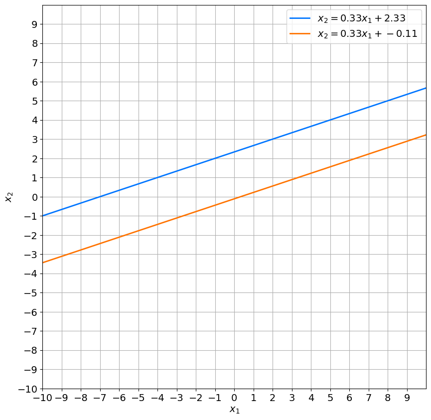

4 - System of Linear Equations with Infinite Number of Solutions¶

Changing free coefficients of the system (5) you can bring it to consistency:

$x^1 + 3x^2 = 7,

$3x^1 + 9x^2 = 21

let’s find the determinant of the corresponding matrix.

b_3 = np.array(
    [7, 21], dtype = np.dtype(float)
)

A_3_system = np.hstack((A_2, b_3.reshape((2, 1))))
print(A_3_system)

[[-1.  3.  7.]
 [ 3. -9. 21.]]

Perform elimination using elementary operations:


# copy() matrix.
A_3_system_res = A_3_system.copy()

# Multiply row 0 by 3 and add it to the row 1.
A_3_system_res[1] = 3 * A_3_system_res[0] + A_3_system_res[1]
print(A_3_system_res)

[[-1.  3.  7.]
 [ 0.  0. 42.]]

Thus from the corresponding linear system

-x^1 + 3x^2 = 7, = 0,

The solutions of linear system(6) are:

x^1 = 3x^2 - 7,

Where x^2 is any real number


plot_lines(A_2_system)

Hybrid Quantum PINNs

Roadmap to Hybrid Quantum Physics-Informed Neural Networks (HQPINNs)

Hybrid Quantum PINNs

🐍 Essential Python Concepts for Learning Hybrid Quantum PINNs